Fit a spectrum
A complete example of fitting an astronomical spectrum is shown below. It is an adaption of ‘fit_a_spectrum’ found in the examples-directory of the software tools, and is followed by a detailed, line-by-line, explanation of the code.
 1observation = OBJ_NEW('AmesPAHdbIDLSuite_Observation', 'myFile', $
 2                       Units=AmesPAHdbIDLSuite_CREATE_OBSERVATION_UNITS_S())
 3
 4observation->AbscissaUnitsTo,1
 5
 6observation->Rebin,5D,/Uniform
 7
 8pahdb = OBJ_NEW('AmesPAHdbIDLSuite')
 9
10transitions = pahdb->getTransitionsByUID( $
11              pahdb->Search("mg=0 o=0 fe=0 si=0 chx=0 ch2=0 c>20"))
12
13transitions->FixedTemperature,600D
14
15transitions->Shift,-15D
16
17spectrum = transitions->Convolve(/Lorentzian, $
18                                 Grid=observation->getGrid(), $
19                                 FWHM=20D)
20
21fit = spectrum->Fit(observation)
22
23OBJ_DESTROY,spectrum
24
25fit->Plot,/Wavelength
26
27fit->Plot,/Wavelength,/Residual
28
29fit->Plot,/Wavelength,/Charge
30
31transitions->Intersect, $
32        fit->getUIDs()
33
34spectrum = transitions->Convolve(/Lorentzian, $
35                                 FWHM=20D, $
36                                 XRange=1D4/[20D, 3D])
37
38coadded = spectrum->CoAdd(Weights=fit->getWeights())
39
40coadded->Plot
41
42OBJ_DESTROY,[coadded, spectrum, fit, transitions, pahdb, observation]
 1import importlib_resources
 2import numpy as np
 3
 4from amespahdbpythonsuite import observation
 5from amespahdbpythonsuite.amespahdb import AmesPAHdb
 6
 7file_path = importlib_resources.files("amespahdbpythonsuite")
 8data_file = file_path / "resources/galaxy_spec.ipac"
 9obs = observation.Observation(data_file)
10
11obs.abscissaunitsto("1/cm")
12
13xml_file = file_path / "resources/pahdb-theoretical_cutdown.xml"
14pahdb = AmesPAHdb(
15    filename=xml_file,
16    check=False,
17    cache=False,
18)
19
20uids = pahdb.search("c>0")
21transitions = pahdb.gettransitionsbyuid(uids)
22
23transitions.cascade(6 * 1.603e-12, multiprocessing=False)
24
25transitions.shift(-15.0)
26
27spectrum = transitions.convolve(
28    grid=obs.getgrid(), fwhm=20.0, gaussian=True, multiprocessing=False
29)
30
31fit = spectrum.fit(obs)
32
33fit.plot(wavelength=True)
34fit.plot(wavelength=True, residual=True)
35fit.plot(wavelength=True, size=True)
36fit.plot(wavelength=True, charge=True)
37fit.plot(wavelength=True, composition=True)
38
39transitions.intersect(fit.getuids())
40
41xrange = 1e4 / np.array([20.0, 3.0])
42
43spectrum = transitions.convolve(
44    xrange=xrange, fwhm=20.0, gaussian=True, multiprocessing=False
45)
46
47coadded = spectrum.coadd(weights=fit.getweights())
48
49coadded.plot()
A line-by-line explanation of the code follows.
lines 1-2: An observation is read from ‘myFile’ and the ‘AmesPAHdbIDLSuite_CREATE_OBSERVATION_UNITS_S’-helper function is called to associate units.
line 4: Observation abscissa units are converted to wavenumber.
line 6: The observation is rebinned onto a uniform grid spaced 5 cm-1.
line 8: The default NASA Ames PAH IR Spectroscopic Database XML-file is loaded.
lines 10-11: The fundamental vibrational transitions from a subset of PAHs are retrieved.
line 13: A FixedTemperature emission model at 600 Kelvin is applied.
line 15: The fundamental vibrational transitions are redshifted 15 cm-1.
line 17: The fundamental vibrational transitions are convolved with Lorentzian profiles having a full-width-at-half-maximum of 20 cm-1 onto the observational grid.
line 21: The observation is fitted with the PAH emission spectra.
line 23: Cleanup of ‘spectrum’.
lines 25-29: Display several aspects of the fit.
line 31: The transitions are intersected with the PAH species in the fit.
line 34: The fundamental vibrational transitions are again convolved with Lorentzian profiles having a full-width-at-half-maximum of 20 cm-1, but now onto a generated grid from 3-20 micron.
line 38: The individual PAH spectra are added using weights retrieved from the fit.
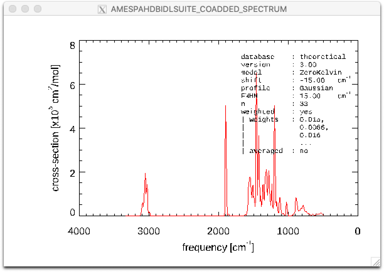
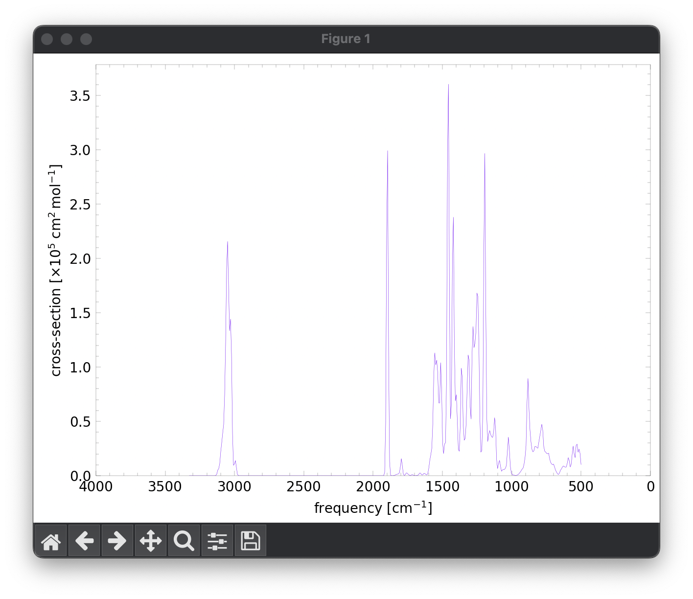
line 40: The coadded spectrum is displayed, revealing the entire 3-20 micron, predicted, PAH spectrum.
line 42: Cleanup.
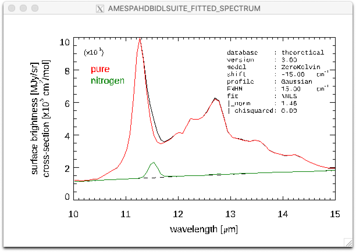
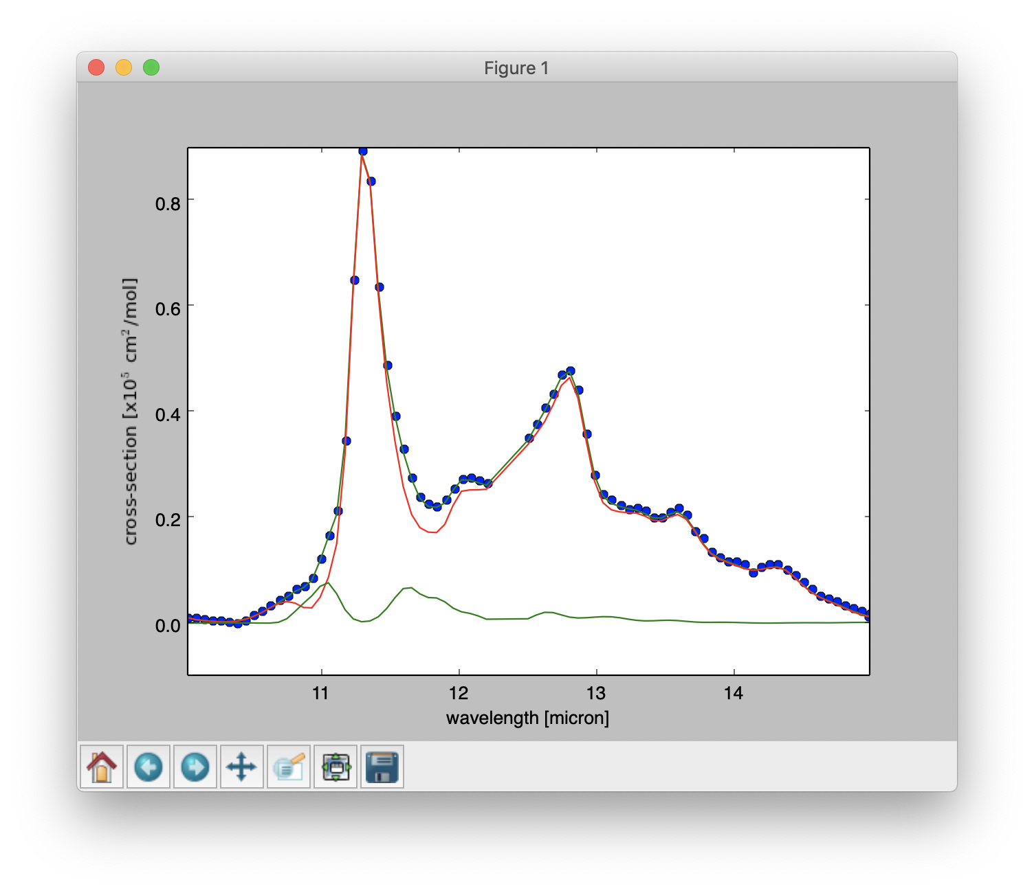
Line 25: A figure is displayed showing the fitted spectrum and its components, as shown below.
lines 1-5: Importing the necessary modules.
lines 7-9: A spectrum included with the suite is loaded.
line 11: Observation abscissa units are converted to wavenumber.
lines 13-18: The cutdown version of the database XML-file included with the suite is loaded.
lines 20-21: The fundamental vibrational transitions of PAHs are retrieved.
line 23: A full temperature cascade emission model at 6 eV is applied.
line 25: The fundamental vibrational transitions are redshifted 15 cm-1.
line 27: The fundamental vibrational transitions are convolved with Lorentzian profiles having a full-width-at-half-maximum of 20 cm-1 onto the observational grid.
line 31: The observation is fitted with the PAH emission spectra.
lines 33-37: Display several aspects of the fit.
line 39: The transitions are intersected with the PAH species in the fit.
line 41: Define a 3-20 micron grid in wavenumbers.
lines 43-45: The fundamental vibrational transitions are again convolved with Lorentzian profiles having a full-width-at-half-maximum of 20 cm:sup:-1, but now onto the generated 3-20 micron grid.
line 47: The individual PAH spectra are added using weights retrieved from the fit.
line 49: The coadded spectrum is displayed, revealing the entire 3-20 micron, predicted, PAH spectrum.
Below some examples of the generated output.
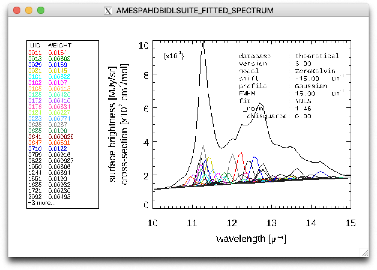
Result of a PAHdb-fit to the 10-15 micron spectrum of NGC 7023 showing the contribution from different PAHs.
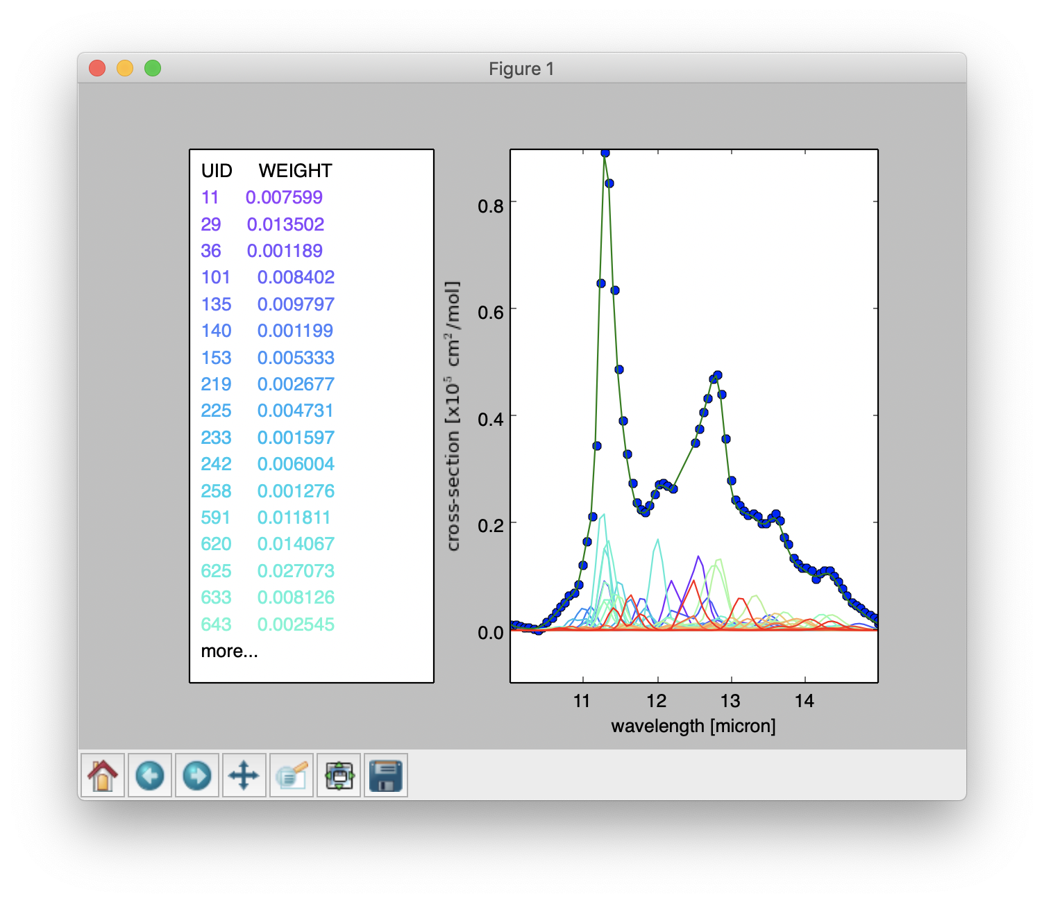
Result of a PAHdb-fit to the 10-15 micron spectrum of NGC 7023 showing the contribution from different PAHs.
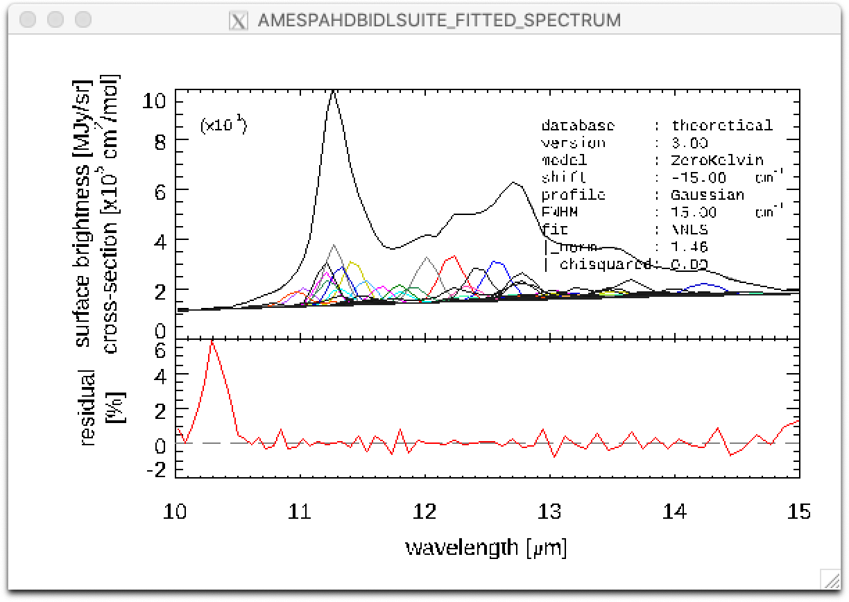
Top: Result of a PAHdb-fit to the 10-15 micron spectrum of NGC 7023 showing the contribution from different PAHs. Bottom: Residual of the fit.
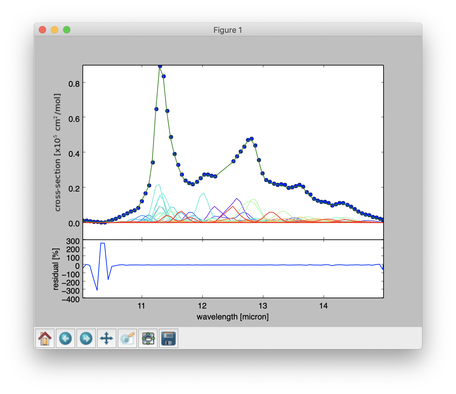
Top: Result of a PAHdb-fit to the 10-15 micron spectrum of NGC 7023 showing the contribution from different PAHs. Bottom: Residual of the fit.
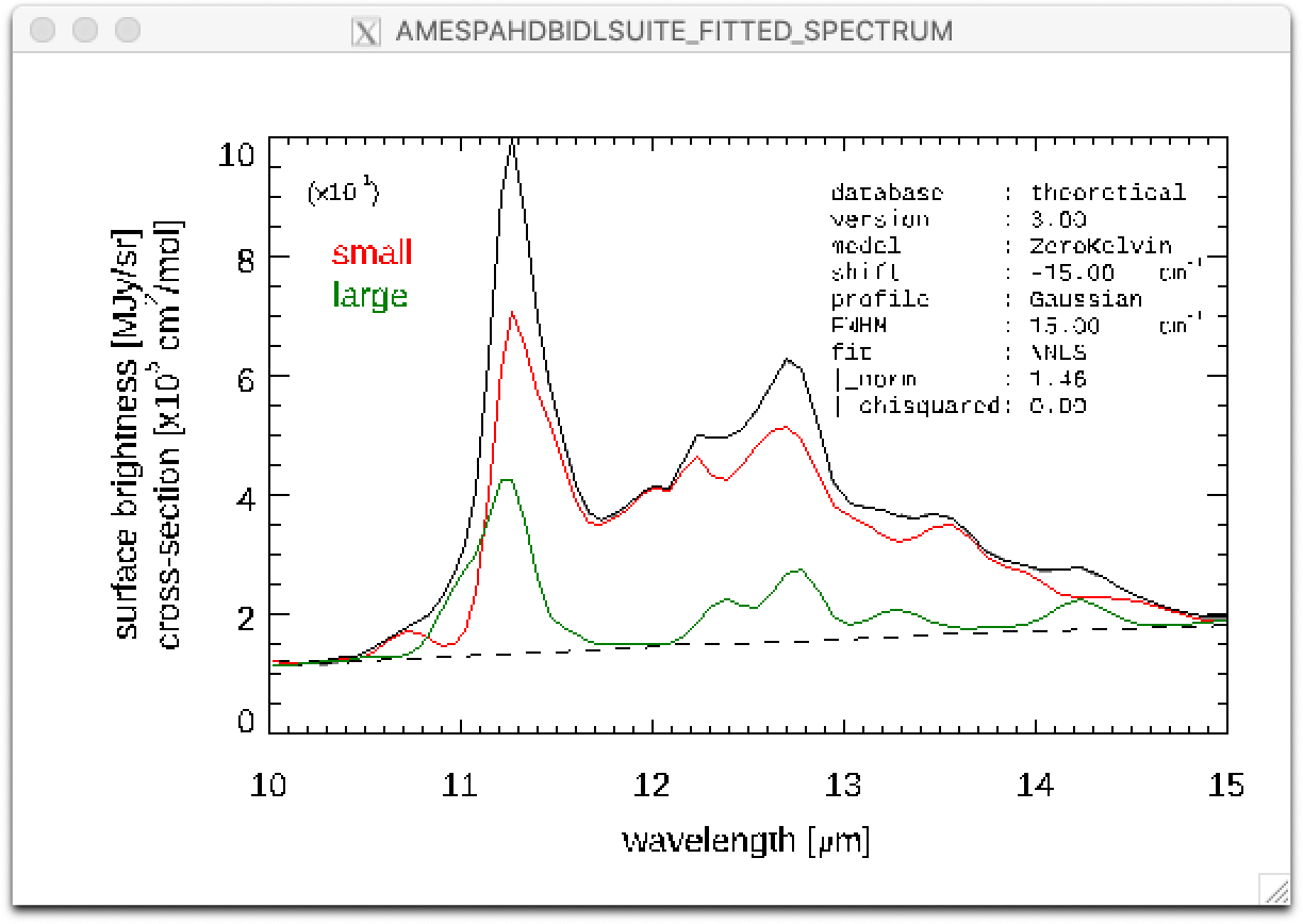
Result of a PAHdb-fit to the 10-15 micron spectrum of NGC 7023 showing the contribution from large and small PAHs.
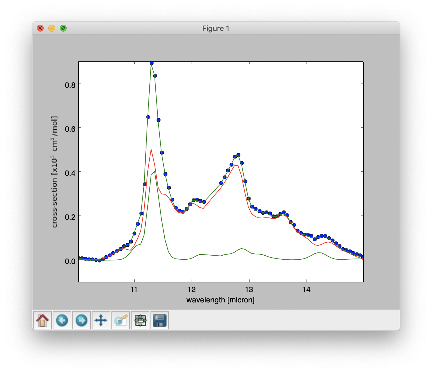
Result of a PAHdb-fit to the 10-15 micron spectrum of NGC 7023 showing the contribution from large and small PAHs.
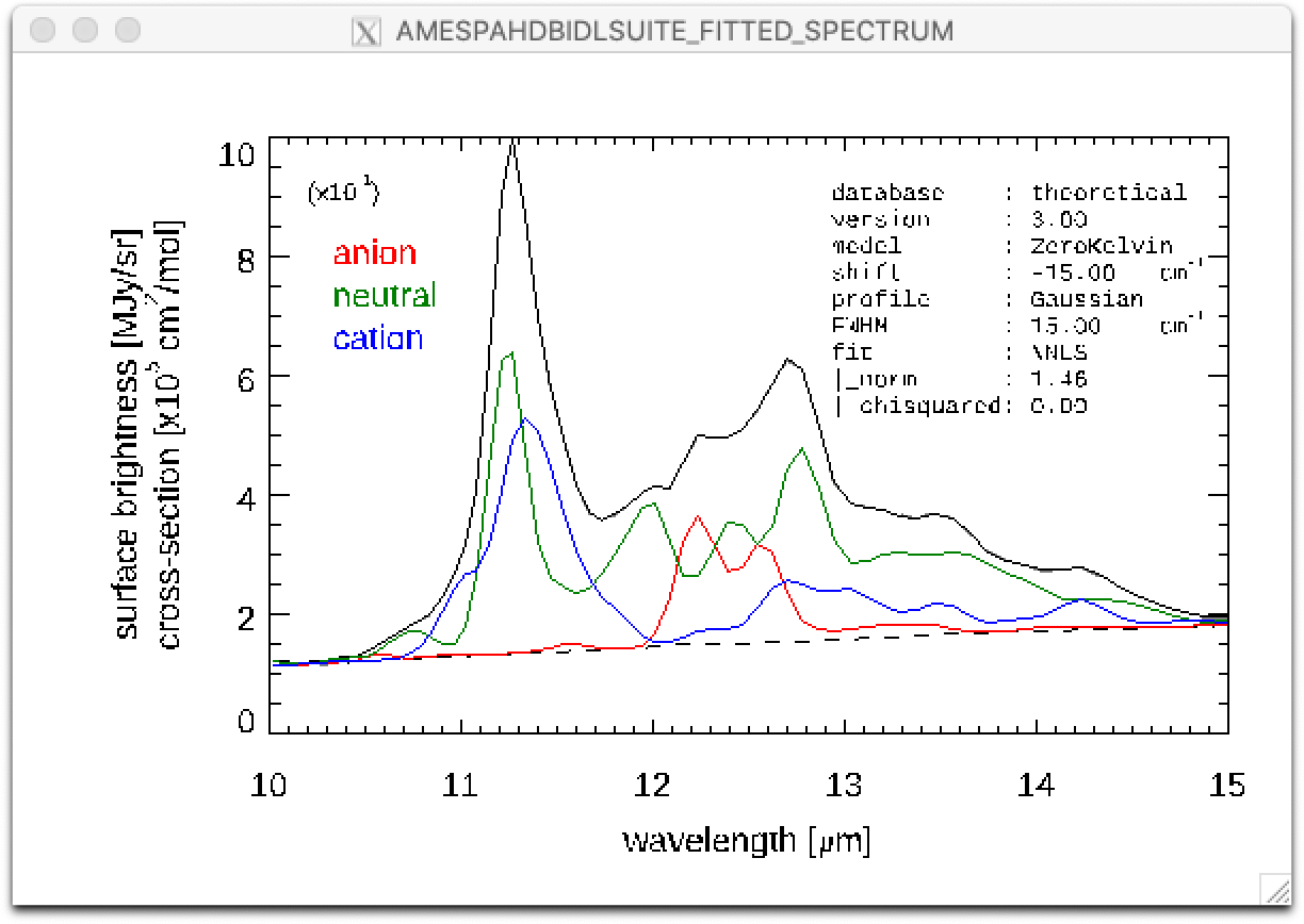
Result of a PAHdb-fit to the 10-15 micron spectrum of NGC 7023 showing the contribution from PAH anions, neutrals and cation.
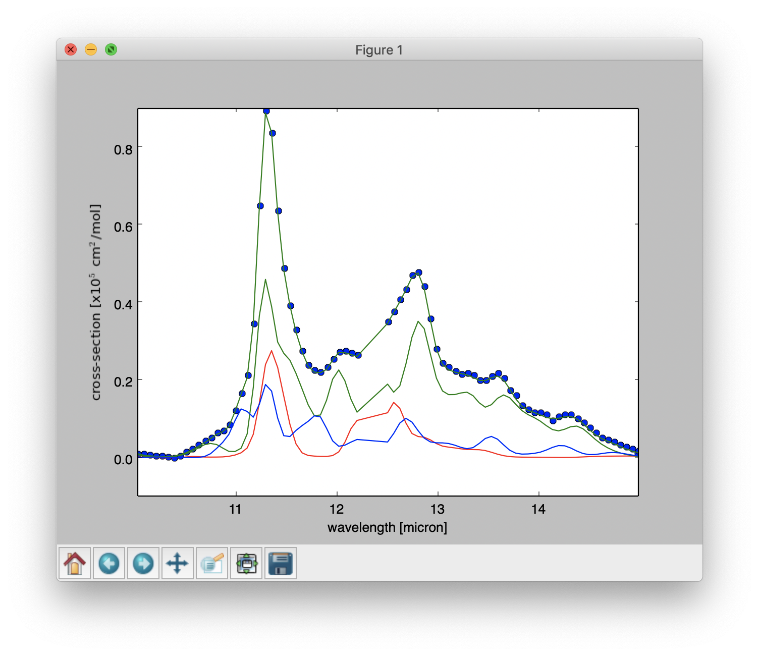
Result of a PAHdb-fit to the 10-15 micron spectrum of NGC 7023 showing the contribution from PAH anions, neutrals and cation.
