Monte Carlo fit a spectrum
A complete example of fitting an astronomical spectrum using a Monte Carlo approach is shown below. It is an adaption of ‘mc_fit_a_spectrum’ found in the examples-directory of the software tools, and is followed by a detailed, line-by-line, explanation of the code.
 1observation = OBJ_NEW('AmesPAHdbIDLSuite_Observation', myFile, $
 2                      Units=AmesPAHdbIDLSuite_CREATE_OBSERVATION_UNITS_S())
 3
 4observation->AbscissaUnitsTo,1
 5
 6pahdb = OBJ_NEW('AmesPAHdbIDLSuite')
 7
 8transitions = pahdb->getTransitionsByUID( $
 9              pahdb->Search("magnesium=0 oxygen=0 iron=0 silicium=0 chx=0 ch2=0 c>20 h>0"))
10
11transitions->Cascade,8D*1.602D-12
12
13transitions->Shift,-15D
14
15spectrum = transitions->Convolve(Grid=observation->getGrid(), $
16                                 FWHM=15D, $
17                                 /Gaussian)
18
19OBJ_DESTROY,[transitions]
20
21mcfit = spectrum->MCFit(observation, 1024)
22
23OBJ_DESTROY,[spectrum]
24
25mcfit->Plot,/Wavelength
26
27mcfit->Plot,/Wavelength,/Size
28
29mcfit->Plot,/Wavelength,/Charge
30
31mcfit->Plot,/Wavelength,/Composition
32
33mcfit->Plot,/DistributionSize,NBins=10L,Min=20,Max=200
34
35OBJ_DESTROY,[mcfit, pahdb, observation]
 1import importlib_resources
 2
 3from amespahdbpythonsuite import observation
 4from amespahdbpythonsuite.amespahdb import AmesPAHdb
 5
 6file_path = importlib_resources.files("amespahdbpythonsuite")
 7data_file = file_path / "resources/galaxy_spec.ipac"
 8obs = observation.Observation(data_file)
 9
10obs.abscissaunitsto("1/cm")
11
12xml_file = file_path / "resources/pahdb-theoretical_cutdown.xml"
13pahdb = AmesPAHdb(
14    filename=xml_file,
15    check=False,
16    cache=False,
17)
18
19uids = pahdb.search("c>0")
20transitions = pahdb.gettransitionsbyuid(uids)
21
22transitions.cascade(8.0 * 1.603e-12, multiprocessing=False)
23
24transitions.shift(-15.0)
25
26spectrum = transitions.convolve(
27    grid=obs.getgrid(), fwhm=15.0, gaussian=True, multiprocessing=False
28)
29
30mcfit = spectrum.mcfit(obs, samples=1024, multiprocessing=False)
31
32mcfit.plot(wavelength=True, residual=True)
33mcfit.plot(wavelength=True, size=True)
34mcfit.plot(wavelength=True, charge=True)
35mcfit.plot(wavelength=True, composition=True)
A line-by-line explanation of the code follows.
lines 1-2: An observation is read from ‘myFile’ and the ‘AmesPAHdbIDLSuite_CREATE_OBSERVATION_UNITS_S’-helper function is called to associate units.
line 4: Observation abscissa units are converted to wavenumber.
line 6: The default NASA Ames PAH IR Spectroscopic Database XML-file is loaded.
lines 8-9: The fundamental vibrational transitions from a subset of PAHs are retrieved.
line 10: A full Cascade emission model at 8 eV is applied.
line 13: The fundamental vibrational transitions are redshifted 15 cm-1.
lines 19-20: The fundamental vibrational transitions are convolved with Gaussian profiles having a full-width-at-half-maximum of 15 cm-1 onto the observational grid.
line 19: Cleanup of ‘transitions’.
line 21: The observation is fitted with the PAH emission spectra using a Monte Carlo approach.
line 23: Cleanup of ‘spectrum’.
line 25-33: Display several aspects of the fit.
line 35: Cleanup.
lines 1-4: Importing the necessary modules.
lines 6-8: A spectrum included with the suite is loaded.
line 10: Observation abscissa units are converted to wavenumber.
line 13: The cutdown version of the database XML-file included with the suite is loaded.
line 15-16: The fundamental vibrational transitions are retrieved.
line 22: A full Cascade emission model at 8 eV is applied.
line 24: The fundamental vibrational transitions are redshifted 15 cm-1.
lines 22-24: The fundamental vibrational transitions are convolved with Gaussian profiles having a full-width-at-half-maximum of 15 cm-1 onto the observational grid.
line 30 The observation is fitted with the PAH emission spectra using a Monte Carlo approach.
line 32-35: Display several aspects of the fit.
Below some examples of the generated output.
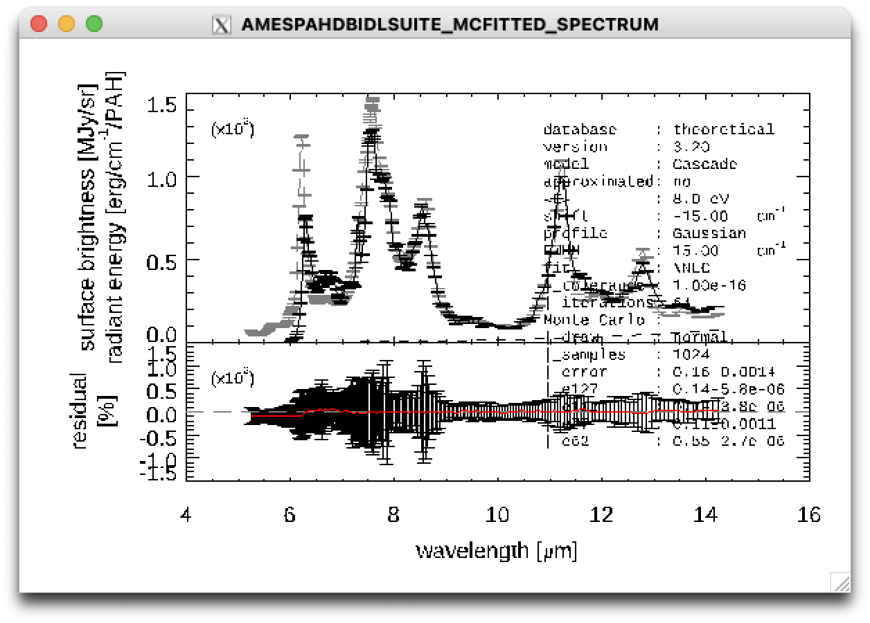
Top: Result of a PAHdb-fit to the 5-15 micron spectrum of NGC 7023. Bottom: Residual of the fit.
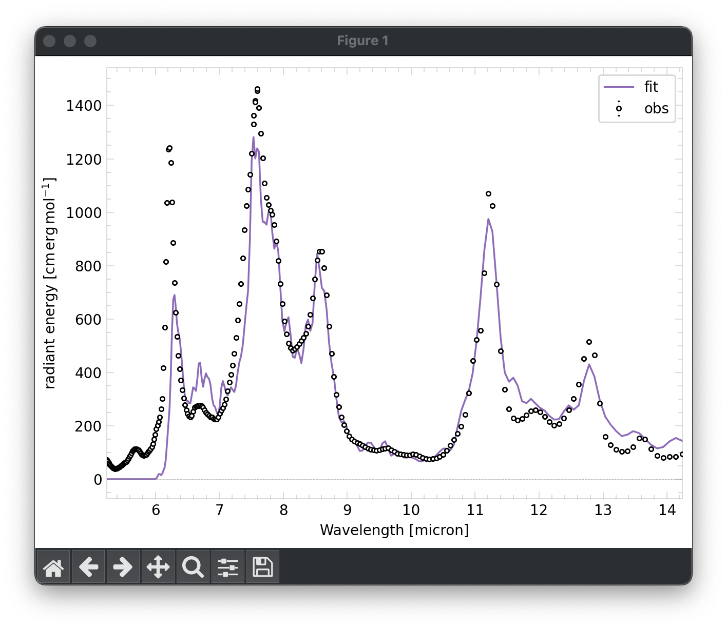
Result of a PAHdb-fit to the 5-15 micron spectrum of NGC 7023.
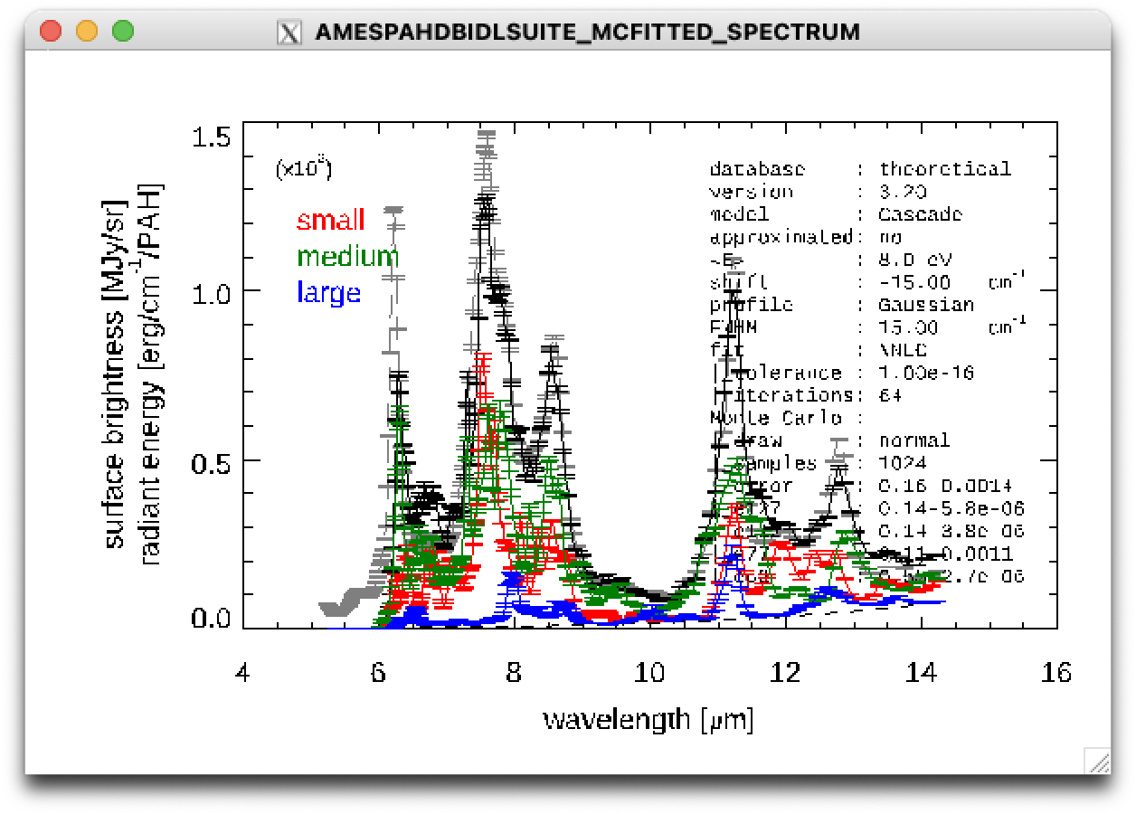
Result of a PAHdb-fit to the 5-15 micron spectrum of NGC 7023 showing the contribution from large, medium, and small PAHs.
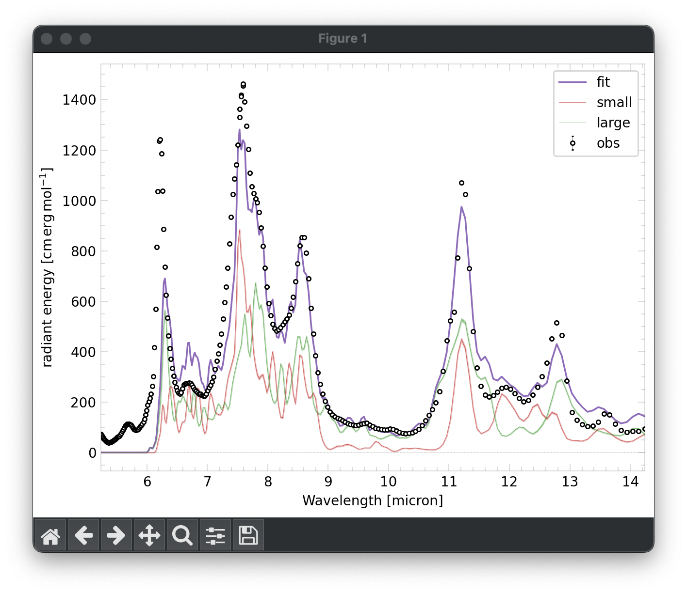
Result of a PAHdb-fit to the 5-15 micron spectrum of NGC 7023 showing the contribution from large and small PAHs.
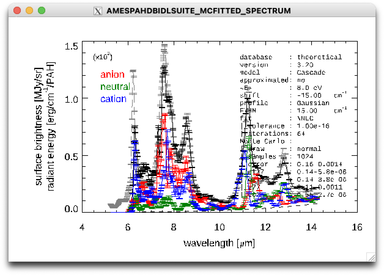
Result of a PAHdb-fit to the 5-15 micron spectrum of NGC 7023 showing the contribution from PAH anions, neutrals and cation.
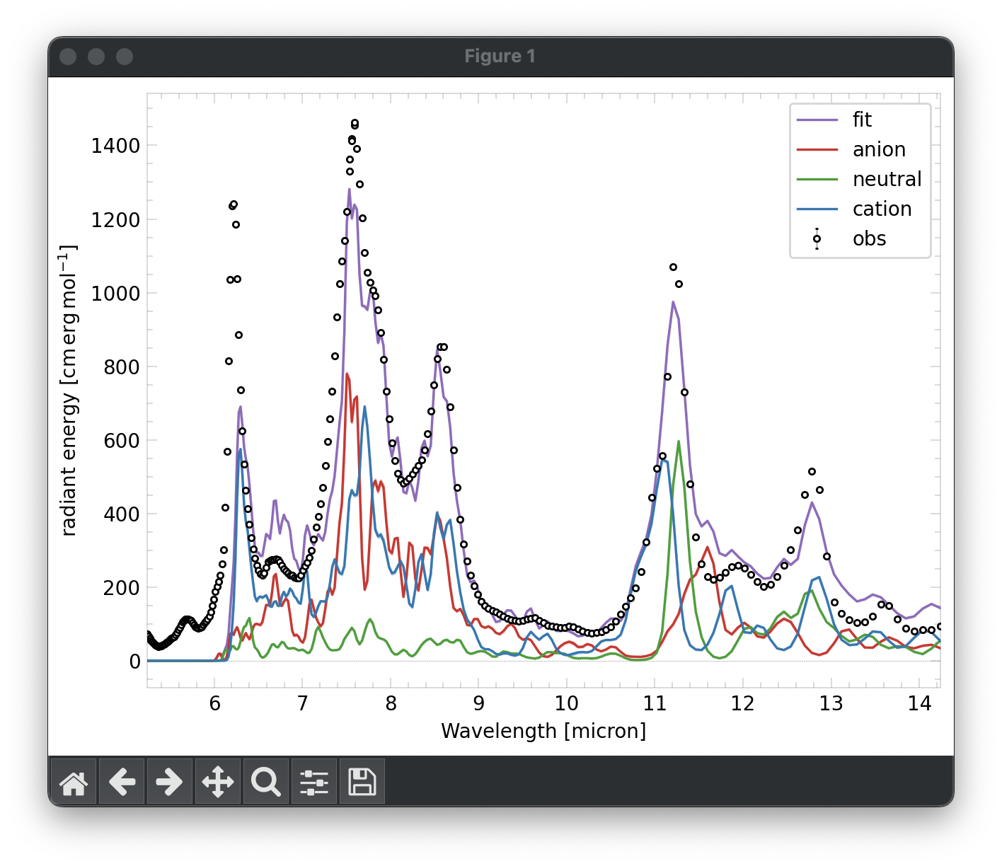
Result of a PAHdb-fit to the 5-15 micron spectrum of NGC 7023 showing the contribution from PAH anions, neutrals and cation.
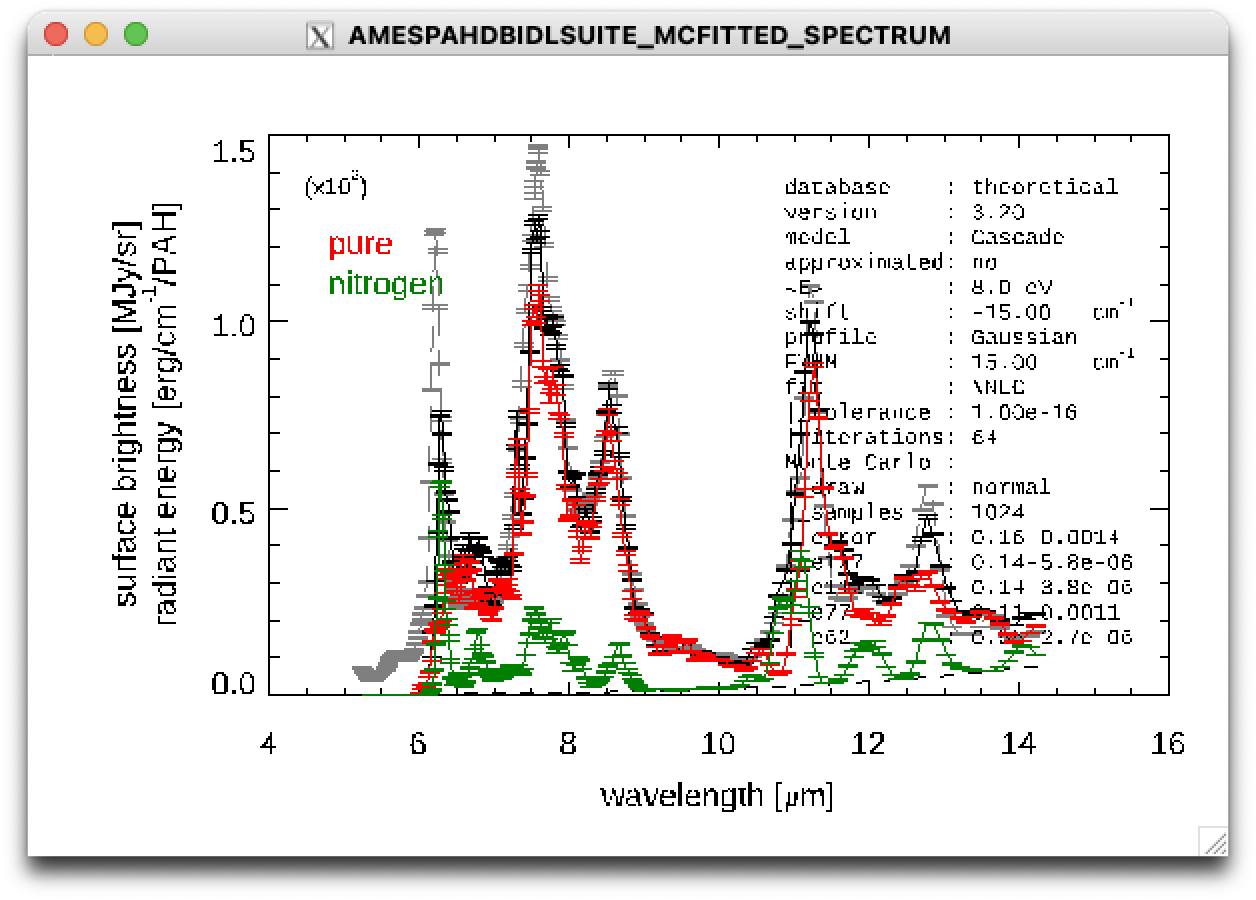
Result of a PAHdb-fit to the 5-15 micron spectrum of NGC 7023 showing the contribution from ‘pure’ and nitrogen containing PAHs (PANHs).
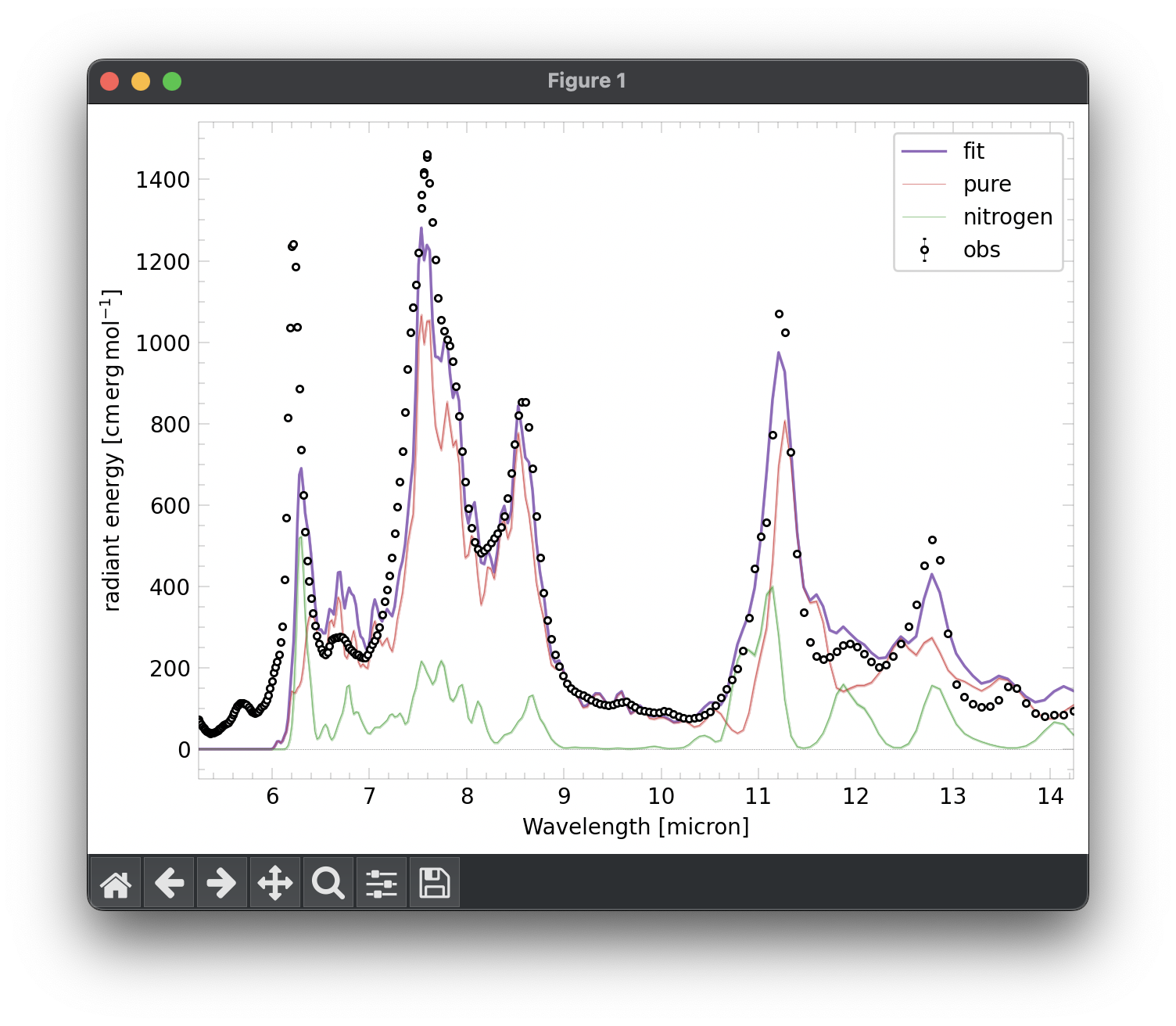
Result of a PAHdb-fit to the 5-15 micron spectrum of NGC 7023 showing the contribution from ‘pure’ and nitrogen containing PAHs (PANHs).
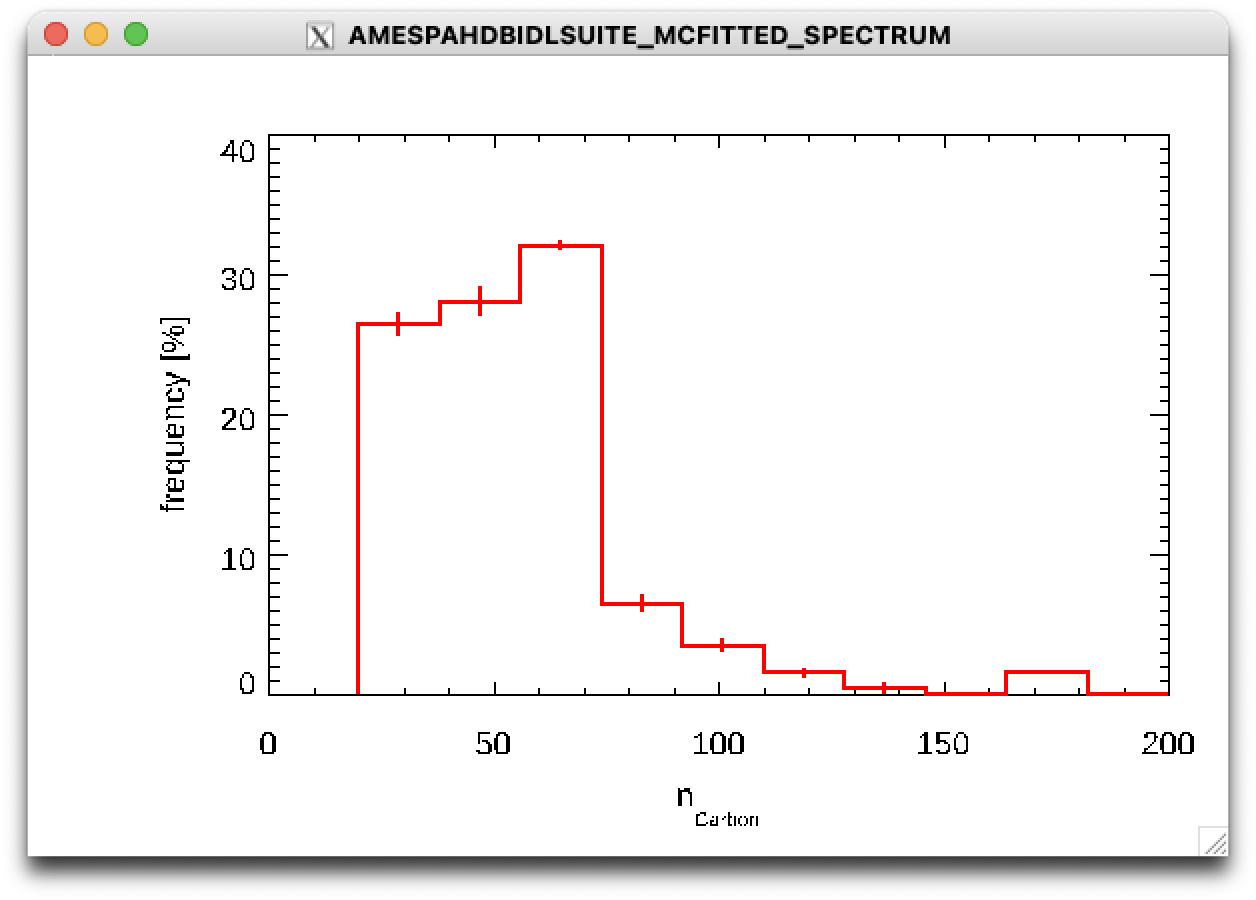
Result of a PAHdb-fit to the 5-15 micron spectrum of NGC 7023 showing the derived PAH size distribution.